Deep Neural Networks (DNNs) are artificial neural networks with many hidden layers. They transform inputs through these layers to learn complex features from data. DNNs excel in tasks like image and speech recognition, and natural language processing. Their success comes from learning from large datasets and using backpropagation to reduce errors. With more computing power and data, DNNs have become essential in deep learning. This post summarizes the SC4001 course at NTU, offering an overview of DNNs based on course notes and my insights.

Chain Rule for Backpropagation of Gradients
- Chain Rule of Differentiation
- Chain Rule in Multi-Dimensions
Basics Concepts of Deep Neural Networks
Process of Using Deep Neural Networks

Chain Rule for Backpropagation of Gradients

Chain Rule of Differentiation

Let $x, y$, and $J \in \mathbf{R}$ be one-dimentional variables, such that:

\[J = g(y), \quad y = f(x)\]

Chain rule can be written as:

\[\frac{dJ}{dx} = \frac{dJ}{dy} \cdot \frac{dy}{dx} \text{ or } \frac{\partial J}{\partial x} = \frac{\partial J}{\partial y} \cdot \frac{\partial y}{\partial x}\] \[\nabla_x J = \frac{\partial y}{\partial x} \cdot \nabla_y J\]

graph LR x --> y y --> J J --> y y --> x J --> x

Chain Rule in Multi-Dimensions

Set $\boldsymbol{x} = (x_1, x_2, \ldots, x_n) \in \mathbf{R}^n$, $\boldsymbol{y} = (y_1, y_2, \ldots, y_k) \in \mathbf{R}^k$, and $J \in \mathbf{R}$, such that:

\[\boldsymbol{J} = g(\boldsymbol{y}), \quad \boldsymbol{y} = f(\boldsymbol{x})\]

Then, the chain rule of differentiation states that:

\[\nabla_{\boldsymbol{x}} \boldsymbol{J} = (\frac{\partial \boldsymbol{y}}{\partial \boldsymbol{x}})^T \cdot \nabla_{\boldsymbol{y}} \boldsymbol{J}\]

where

\[\nabla_{\boldsymbol{x}} \boldsymbol{J} = \frac{\partial \boldsymbol{J}}{\partial \boldsymbol{x}} = \begin{bmatrix} \frac{\partial J}{\partial x_1} \\ \frac{\partial J}{\partial x_2} \\ \vdots \\ \frac{\partial J_1}{\partial x_n} \\ \end{bmatrix} \qquad \nabla_{\boldsymbol{y}} \boldsymbol{J} = \frac{\partial \boldsymbol{J}}{\partial \boldsymbol{y}} = \begin{bmatrix} \frac{\partial J}{\partial y_1} \\ \frac{\partial J}{\partial y_2} \\ \vdots \\ \frac{\partial J}{\partial y_k} \\ \end{bmatrix}\] \[\frac{\partial \boldsymbol{y}}{\partial \boldsymbol{x}} = \begin{bmatrix} \frac{\partial y_1}{\partial x_1} & \frac{\partial y_1}{\partial x_2} & \cdots & \frac{\partial y_1}{\partial x_n} \\ \frac{\partial y_2}{\partial x_1} & \frac{\partial y_2}{\partial x_2} & \cdots & \frac{\partial y_2}{\partial x_n} \\ \vdots & \vdots & \ddots & \vdots \\ \frac{\partial y_k}{\partial x_1} & \frac{\partial y_k}{\partial x_2} & \cdots & \frac{\partial y_k}{\partial x_n} \\ \end{bmatrix}\]

The matrix $\frac{\partial \boldsymbol{y}}{\partial \boldsymbol{x}}$ is called the Jacobian matrix of function $f$ where $\boldsymbol{y} = f(\boldsymbol{x})$.

Note that differentiation of a scalar by a vector results in a vector and differentiation of a vector by a vector results in a matrix.

Look at the following example, set $\boldsymbol{x} = (x_1, x_2, x_3) \in \mathbf{R}^3$, and $\boldsymbol{y} = (y_1, y_2) \in \mathbf{R}^2$, such that:

\[f(\boldsymbol{x}) = \boldsymbol{y} = \begin{bmatrix} y_1 \\ y_2 \end{bmatrix} = \begin{bmatrix} 5 - 2 x_1 + 3 x_3 \\ x_1 + 5 x_2^2 + x_3^3 - 1 \end{bmatrix}\]

We can compute each term of the Jacobian matrix:

\[\frac{\partial \boldsymbol{y}}{\partial \boldsymbol{x}} = \begin{bmatrix} \frac{\partial y_1}{\partial x_1} & \frac{\partial y_1}{\partial x_2} & \frac{\partial y_1}{\partial x_3} \\ \frac{\partial y_2}{\partial x_1} & \frac{\partial y_2}{\partial x_2} & \frac{\partial y_2}{\partial x_3} \end{bmatrix} = \begin{bmatrix} -2 & 0 & 3 \\ 1 & 10 x_2 & 3 x_3^2 \end{bmatrix}\]

Basics Concepts of Deep Neural Networks

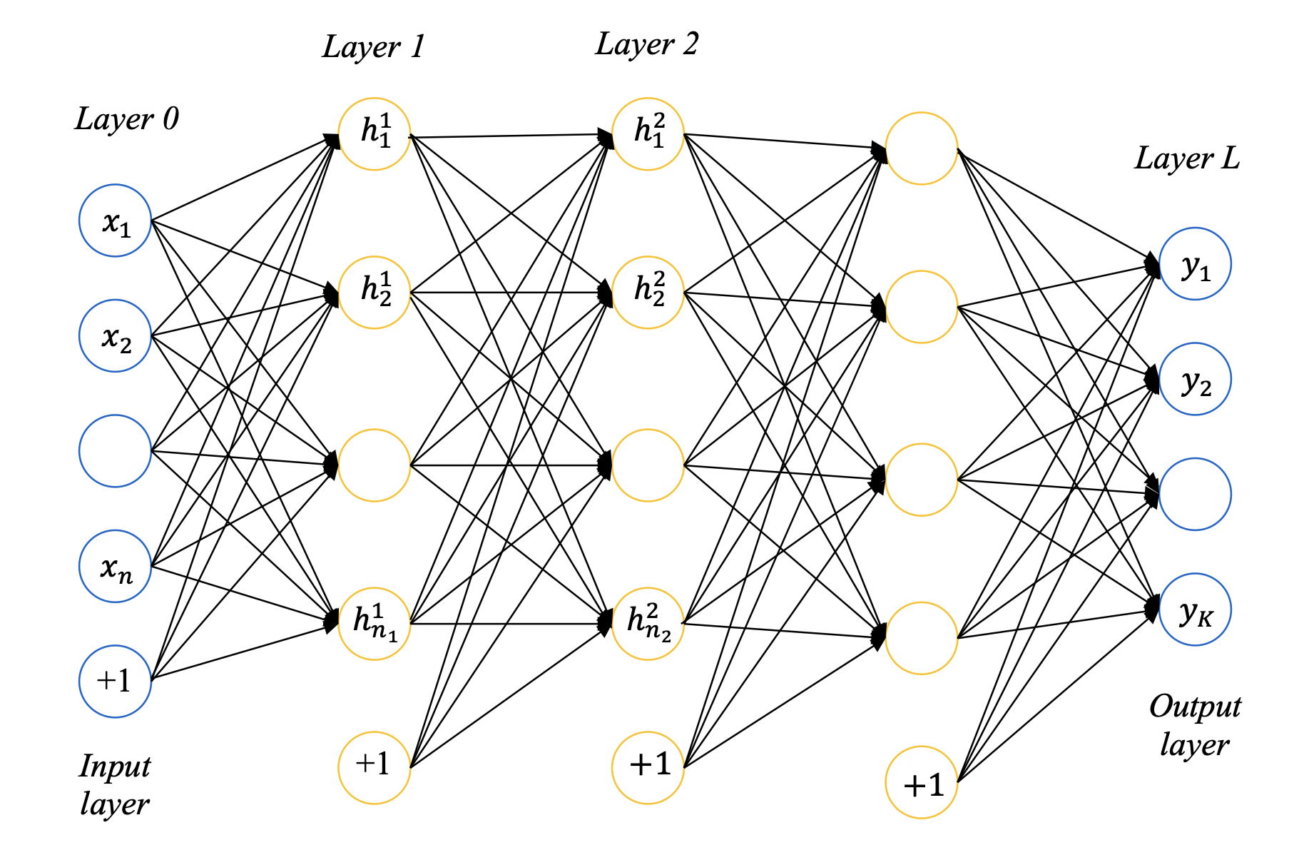
Feedforward networks (FFN) consists of several layers of neurons where activations propagate from input layer to output layer. The layers between the input layer and output layer are referred to as hidden layers.

Deep Neural Network Example — deep neural network example

The number of layers is referred to as the depth of the feedforward network. When a network has many hidden layers of neurons, feedforward networks are referred to as deep neural networks (DNN). Learning in deep neural networks is referred to as deep learning. The number of neurons in a layer is referred to as the width of that layer.

The hidden layers are usually composed of perceptron layers or ReLU layers and the output layer is usually:

A linear layer for regression
A softmax layer for classification

Width of Hidden Layers

The width of hidden layers has a significant impact on the performance of the network. With more parameters, the network is capable of remembering the training patterns better, but it may also lose its generalization ability on unseen data. As a result, the test error may decrease initially with more hidden units, but it may also increase beyond a certain point. Determining the optimal number of hidden units is often an empirical process, requiring trial and error.

Depth of Deep Neural Networks

The depth of a deep neural network is dependent on the amount of available training data. Deeper networks have more parameters (weights and biases) to learn, and thus require more data to train. With sufficient training data, deeper networks can learn complex mappings more accurately. The optimal number of layers is often determined empirically, by finding the architecture that minimizes the error (training, testing and validation).

Normalization of Inputs

If inputs have similar variations, better approximation of inputs or prediction of outputs is achieved. Mainly, there are two approaches to normalization of inputs.

Suppose $i$th input $x_i \in [x_{i,min}, x_{i,max}]$ and has a mean $\mu_i$ and a standard deviation $\sigma_i$. If $\widetilde{x}$ denotes the normalized input, two approaches are:

Scaling the inputs such that $\widetilde{x} \in [0, 1]$:

\[\widetilde{x}_i = \frac{x_i - x_{i, min}}{x_{i, max} - x_{i, min}}\]

Normalization the inputs such that $\widetilde{x} \sim \mathcal{N}(0, 1)$:

\[\widetilde{x}_i = \frac{x_i - \mu_i}{\sigma_i}\]

Normalization of Outputs

The normalization of outputs depends on the final activation function used.

For linear activation function, the convergence is usually improved if each output is normalized to have zero mean and unit standard deviation:

\[\widetilde{y}_k = \frac{y_k - \mu_k}{\sigma_k}\]

For sigmiod activation function, I think the normalization is not that necessary. But we can till scale $\widetilde{y}_k \in [0, 1]$:

\[\widetilde{y}_k = \frac{y_k - y_{k,min}}{y_{k,max} - y_{k,min}}\]

Gradient Descent Optimization

Set $P$ to be the number of training samples and $B$ to be the batch size. The choice of batch size $B$ in gradient descent has a significant impact on the training process. In this subsection, we’ll explore the three main forms of gradient descent and discuss how batch size affects computation.

Forms of Gradient Descent	Batch Size	Advantages	Disadvantages
Stochastic Gradient Descent	$B = 1$	Fast computation, low memory usage, suitable for online learning	Noisy gradient directions, unstable convergence
Batch Gradient Descent	$B = P$	Accurate gradient directions, stable convergence	Slow computation, high memory requirements, no parallelization
Mini-batch Stochastic Gradient Descent	$1 < B < P$	Compromise between computation efficiency and convergence stability, suitable for modern hardware with parallel acceleration

The computation time versus batch size exhibits a U-shaped curve, where the optimal batch size is located at the minimum point. A larger batch size can take advantage of parallelization and memory caching optimization, but may also result in increased computation time per iteration and memory pressure due to the limited hardware cache capacity. In practice, the optimal batch size should be determined based on the hardware cache size and computation capabilities, and adjusted dynamically according to the specific task requirements and training conditions.

Parallelization: Parallelization refers to the process of dividing a computational task into smaller, independent sub-tasks that can be executed simultaneously across multiple processors or cores. This approach can significantly reduce computation time by leveraging the capabilities of modern multi-core processors and distributed computing systems. In the context of gradient descent, parallelization can be used to compute gradients for multiple data points or mini-batches concurrently, improving the efficiency of the training process.
Memory Caching: Memory caching is a technique used to temporarily store frequently accessed data in a fast-access storage layer, known as a cache, to reduce latency and improve performance. Caches are typically smaller but faster than main memory, allowing for quicker retrieval of data. In machine learning, caching can be used to store intermediate results, model parameters, or frequently used data points, reducing the time spent on data transfer and computation. Effective memory caching can help manage the memory pressure caused by large batch sizes during training.

For SGD, it is desirable to randomly sample the patterns from training data in each epoch. To efficiently sample blocks, the training patterns are shuffled at the beginning of every training epoch and then blocks are sequentially fetched from memory. Typical batch sizes: $16, 32, 64, 128, 256, \dots$

Process of Using Deep Neural Networks

The development of deep neural networks (DNNs) has a long history, dating back to the 1940s and 1950s when the first artificial neural networks were developed. The first neural network simulator, called the “Threshold Logic Unit,” was developed in 1958. The 1960s and 1970s saw the development of the first multi-layer perceptrons and the introduction of the backpropagation algorithm. Later, the development of DNNs was hindered by the lack of computational power and data. However, with the advent of large-scale datasets and significant improvements in computing hardware, DNNs have seen a resurgence in popularity since the 2000s. In this section, we will explore how DNNs are used in practice and provide a brief overview of their notations.

DNN Notations

Before we start, let’s have a short definition of DNN notations.

Layer	Width	Weights and Biases	Synaptic Input	Activation Function	Output	Desired Output
Input layer $l=0$	$n$		Input $\boldsymbol{x}$, $\boldsymbol{X}$
Hidden layers $l=1,2,\dots,L-1$	$n_l$	Weight matrix $\boldsymbol{W}_l$, bias vector $\boldsymbol{b}_l$	Synaptic input $\boldsymbol{u}_l$, $\boldsymbol{U}_l$	Activation function $f_l$	Output $\boldsymbol{h}_l$, $\boldsymbol{H}_l$
Output layer $l=L$	$K$		Synaptic input $\boldsymbol{u}_L$, $\boldsymbol{U}_L$	Activation function $f_L$	Output $\boldsymbol{y}$, $\boldsymbol{Y}$	Desired output $\boldsymbol{d}$, $\boldsymbol{D}$

Forward propagation of activation

For one single pattern, the forward propagation of activation is:

\[\begin{align*} &\text{Input } \boldsymbol{x}, \boldsymbol{d}\\ &\boldsymbol{u}_1 = \boldsymbol{W}_1^T\boldsymbol{x} + \boldsymbol{b}_1\\ &\text{For layers } l = 1, 2, \dots, L - 1:\\ &\qquad\boldsymbol{h}_l = f_l(\boldsymbol{u}_l)\\ &\qquad\boldsymbol{u}_{l+1} = \boldsymbol{W}_{l+1}^T\boldsymbol{h}_l + \boldsymbol{b}_{l+1}\\ &\boldsymbol{y} = f_L(\boldsymbol{u}_L) \end{align*}\]

For batch of patterns, the forward propagation of activation is similar, except that the input is replaced by the batch of patterns, and the output is replaced by the batch of outputs:

\[\begin{align*} &\text{Input } \boldsymbol{X}, \boldsymbol{D}\\ &\boldsymbol{U}_1 = \boldsymbol{W}_1^T\boldsymbol{X} + \boldsymbol{b}_1\\ &\text{For layers } l = 1, 2, \dots, L - 1:\\ &\qquad\boldsymbol{H}_l = f_l(\boldsymbol{U}_l)\\ &\qquad\boldsymbol{U}_{l+1} = \boldsymbol{W}_{l+1}^T\boldsymbol{H}_l + \boldsymbol{b}_{l+1}\\ &\boldsymbol{Y} = f_L(\boldsymbol{U}_L) \end{align*}\]

Back-propagation of gradients

For one pattern, the back-propagation of gradients is as follows:

If $l = L$

\[\nabla_{\boldsymbol{u}^l} J = \begin{cases} - (\boldsymbol{d} - \boldsymbol{y}) & \text{if linear activation}\\ - (1 [\boldsymbol{k} = d] - f^l(\boldsymbol{u}^l)) & \text{if softmax activation} \end{cases}\]

Else

\[\nabla_{\boldsymbol{u}^l} J = \boldsymbol{W}^{l+1} \nabla_{\boldsymbol{u}^{l+1}} J \cdot f^l(\boldsymbol{u}^l)\]

And

\[\begin{cases} \nabla_{\boldsymbol{b}^l} J = \nabla_{\boldsymbol{u}^l} J\\ \nabla_{\boldsymbol{W}^l} J = \boldsymbol{h}^{l-1} \cdot (\nabla_{\boldsymbol{u}^l} J)^T \end{cases}\]

By iterating the above, gradients are backpropagated from the output layer to the input layer. Similar for batch of patterns.

If $l = L$

\[\nabla_{\boldsymbol{U}^l} J = \begin{cases} - (\boldsymbol{D} - \boldsymbol{Y}) & \text{if linear activation}\\ - (\boldsymbol{K} - f^l(\boldsymbol{U}^l)) & \text{if softmax activation} \end{cases}\]