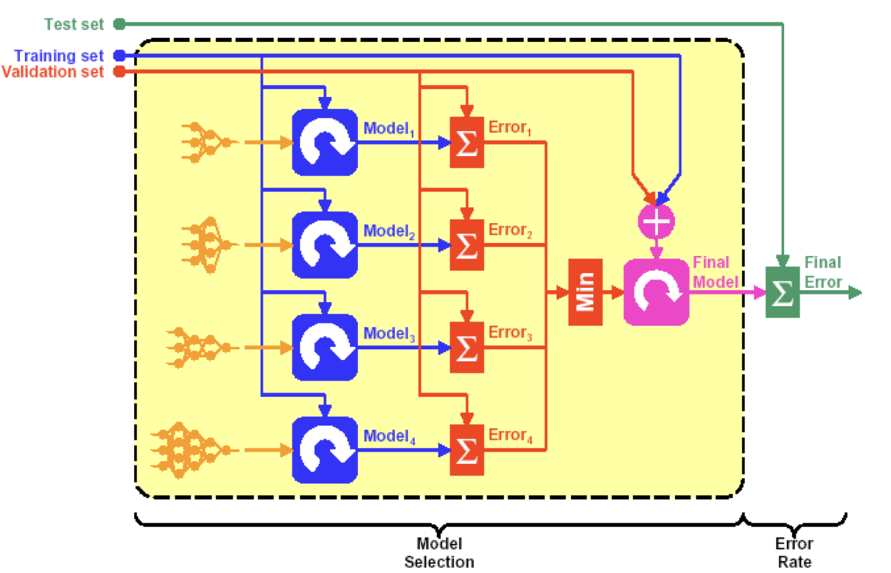
In neural networks, there exist several free parameters: learning rate, batch size, number of layers, number of neurons, etc. We are faced with the problem of selecting the best model for a given regression or classification problem. There are various ways to do so. We can either select the best model with the best parameter value. This post is a lecture notes of the SC4001 course at NTU, covering model selection and overfitting.

Table of Contents

• Model Performance Evaluation
  • Evaluation Metrics
  • True Error and Transparent Error
• Validation
  • Holdout Method
  • Random Sampling Methods
    • $K$ Data Splits Random SubSampling
    • $K$-fold Cross-Validation
    • Leave One Out Cross-Validation
  • Three-way Data Splites
• Overfitting and Underfitting
  • Early Stopping
  • Regularization of Weights
  • Dropout

Model Performance Evaluation

Evaluation Metrics

For regression problem, we can use Mean Square Error/Root Mean Square Error. A measure of the deviation from actual:

where $d_{p,k}$ is the actual value of the $k^{th}$ output of the $p^{th}$ sample, and $y_{p,k}$ is the predicted value of the $k^{th}$ output of the $p^{th}$ sample.

For classification problem, we can use Classification Error, which is defined as the number of misclassified samples divided by the total number of samples:

Here $[\text{Condition Expression}]$ is the indicator function.

True Error and Transparent Error

• True Error: the error that will be obtained in use (i.e., over the whole sample space). What we want to optimize but unknown.
• Apparent Error (Training Error): the error on the training data. What the learning algorithm tries to optimize.

However, the apparent error is not always a good estimate of the true error. It is just an optimistic measure of it.

Test Error (Out-of-Sample Error): an estimate of the true error obtained by testing the network on some independent data. Generally, a larger test set helps provide a greater confidence on the accuracy of the estimate.

Choose the model with the best fit to the data means Choose the model that provides the lowest error rate on the entire sample population. Of course, that error rate is the true error rate.

However, to choose a model, we must first know how to estimate the error of a model.

Validation

In real applications, we only have access to a finite set of examples, usually smaller than we wanted.

Validation is the approach to use the entire example data available to build the model and estimate the error rate. The validation uses a part of the data to select the model, which is known as the validation set.

Validation attempts to solve fundamental problems encountered:

• To avoid overfitting on training data. It is not uncommon to have $100\%$ correct classification on training data.
• There is no way of knowing how well the model performs on unseen data. To generalize well.
• The error rate estimate will be overly optimistic (usually lower than the true error rate). Need to get an unbiased estimate.

A common approach is to split the entire dataset into three parts: a training set, a validation set, and a test set. This helps to avoid overfitting and underfitting. Some popular methods for splitting the data are:

• Holdout: split the data into two parts, one for training and one for validation (e.g. $\frac{2}{3}$ for training and $\frac{1}{3}$ for validation)
• Resampling Techniques
  • Random Subsampling
  • K-fold Cross-Validation
  • Leave one out Cross-Validation
• Three-way data splites (training, validation and test)

Holdout Method

Split entire dataset into two sets:

• Training Set ($\frac{2}{3}$): used to train the classifier.
• Testing Set ($\frac{1}{3}$): used to estimate the error rate of the trained classifier on unseen data samples.

The holdout method has two basic drawbacks:

• By setting some samples for testing, the training dataset becomes smaller.
• Use of a single train-and-test experiment, could lead to misleading estimate if an “unfortunate” split happen.

Random Sampling Methods

Limitations of the holdout can be overcome with a family of resampling methods at the expense of more computations.

$K$ Data Splits Random SubSampling

Random Subsampling performs $K$ data splits of the dataset for training and testing.

Each split randomly selects a (fixed) number of examples. For each data split we retrain the classifier from scratch with the training data. Let the error estimate obtained for 𝑖th split (experiments) be $e_i$.

$K$-fold Cross-Validation

To create a $$K$-fold partition of the the dataset: for each of $K$ experiments, use $K-1$ folds for training and the remaining one-fold for testing.

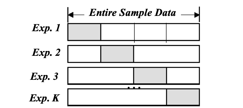
$K$-fold cross validation is similar to K Data Splits Random Subsampling. The advantage of $K$-Fold Cross validation is that all examples in the dataset are eventually used for both training and testing.

Leave One Out Cross-Validation

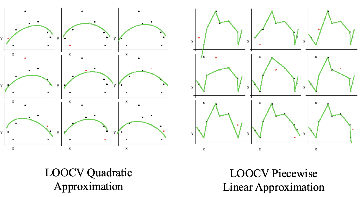
Leave-One-Out is the degenerate case of $K$-Fold Cross Validation, where K is chosen as the total number of examples.

• For a dataset with $N$ examples, perform $N$ experiments, i.e., $N=K$.
• For each experiment use $N-1$ examples for training and the remaining one example for testing

Three-way Data Splites

Dataset is partitioned in to training set, validation set, and testing set.

If model selection and true error estimates are to be computed simultaneously, the data needs to be divided into three disjoint sets:

• Training Set: examples for learning to fit the parameters of several possible classifiers. In the case of DNN, we would use the training set to find the “optimal” weights with the gradient descent rule.
• Validation Set: examples to determine the error $e_m$ of different models $m$, using the validation set. The optimal model $m^*$ is given by

• Training and Validation Set: combine examples used to re-train/redesign model $m^*$, and find new “optimal” weights and biases.
• Test Set: examples used only to assess the performance of a trained model $m^*$. We will use the test data to estimate the error rate after we have trained the final model with train + validation data.

The error rate estimate of the final model on validation data will be biased (smaller than the true error rate) since the validation set is also used to select in the process of final model selection. After assessing the final model, an independent test set is required to estimate the performance of the final model.

Overfitting and Underfitting

Complex models, which have numerous adjustable weights and biases, are:

• More likely to successfully complete the required task.
• More prone to memorizing the training data without truly solving the task.

Simple models, on the other hand, are:

• More likely to generalize well across the entire sample space, given their simplicity.
• Potentially inadequate in learning the problem thoroughly.

This highlights a fundamental trade-off:

• A model that is too simple may underfit, failing to perform the task due to insufficient parameters (e.g., using only 5 hidden neurons).
• Conversely, a model that is too complex may overfit, struggling to generalize well from small and noisy datasets (e.g., using 20 hidden neurons).

Overfitting is one of the problems that occur during training of neural networks, which drives the training error of the network to a very small value at the expense of the test error. The network learns to respond correctly to the training inputs by remembering them too much but is unable to generalize to produce correct outputs to novel inputs. It happens when the amount of training data is inadequate in comparison to the number of network parameters to learn. Also occurs when the weights and biases become too large and are fine-tuned to remember the training patterns too much. Training too many epochs is another cause of overfitting even if the model is right.

But luckily, we can use Early Stopping, Regularization, and Dropout to prevent overfitting.

Early Stopping

Training of the network is to be stopped when the validation error starts increasing. Early stopping can be used in test/validation by stopping when the validation error is minimum.

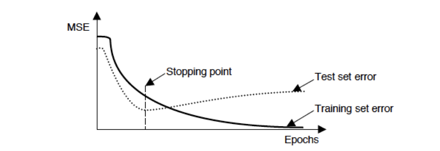
In practice we can write a class to track the validation error and stop training when the error starts increasing:

class EarlyStopper:
    def __init__(self, patience=5, min_delta=0):
        self.patience = patience
        self.min_delta = min_delta
        self.counter = 0
        self.min_validation_loss = np.inf

    def early_stop(self, validation_loss):
        if validation_loss < self.min_validation_loss:
            self.min_validation_loss = validation_loss
            self.counter = 0
        elif validation_loss > (self.min_validation_loss + self.min_delta):
            self.counter += 1
        if self.counter >= self.patience:
            return True
        return False

where patience is the number of epochs to wait for the validation error to improve before stopping and min_delta is the minimum change in the validation error to consider as improvement. In the training process like:

for t in range(max_epochs):
    model.train()
    train_loss, train_correct = train_loop(train_dataloader, model, loss_fn, optimizer)
    
    model.eval()
    test_loss, test_correct = test_loop(test_dataloader, model, loss_fn)
    
    if early_stopper.early_stop(test_loss):
        print("Done!")
        break

Regularization of Weights

During overfitting, some weights attain large values to reduce training error, jeopardizing its ability to generalizing. In order to avoid this, a penalty term (regularization term) is added to the cost function.

For a network with weights $\boldsymbol{W} = {w_{i, j}}$, the penalized cost function $J_1(\boldsymbol{W})$ is defined as:

where $J$ is the original (standard) cost function (e.g., cross-entropy), and $\beta_1$ and $\beta_2$ are the regularization (penalty) parameters,

• $L^1$ - norm is the term $\sum_{i, j} |w_{i, j}|$, the sparsity of the weights
• $L^2$ - norm is the term $\sum_{i, j} w_{i, j}^2$, the quantity of the weights

We have facts that regularization is usually not applied on bias terms, and $L^2$ regularization is most popular on weights. The gradient decent procedure ($L^2$ regularization) is like:

where $2 \alpha \beta_2$ can be written as $\beta$, which is also known as weight decay parameter. The weight matrix is weighted by decay parameter and added to the gradient term. Following is a simple example of training process of a network with and without weight decay:

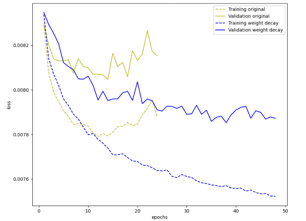
where the process is about DNN with $[3072, 400, 400, 400, 10]$ architecture. Let’s implement $L^2$ regularization with $\beta = 0.0001$ on dataset CIFAR-10.

Dropout

Overfitting can be avoided by training only a fraction of weights in each iteration. The key idea of dropouts is to randomly drop neurons (along with their connections) from the networks during training. This prevents neurons from co-adapting and thereby reduces overfitting.

At the training time, the units (neurons) are dropped randomly at probability $p$ and presented to the next layer with weight $W$. In other words, only $1 − p$ fraction of neurons will be present at the training time.

This results in a scenario that at test time, the weights are always present and presented to the network with the weights multiplied by probability $1 − p$. That is, the output at the test time need to be scaled by $\frac{1}{1 − p}$.

Dropout ratio is the fraction of neurons to be dropped out at one forward step. In Pytorch, dropout ratio ($p$) has to be specified with nn.Dropout() after the activation function. Here is an example of dropout in Pytorch (classification task on CIFAR-10):

class NeuralNetwork_dropout(nn.Module):
    def __init__(self, hidden_size = 100, drop_out=0.5):
        super(NeuralNetwork_dropout, self).__init__()
        self.flatten = nn.Flatten()
        self.linear_relu_stack = nn.Sequential(
            nn.Linear(32*32*3, hidden_size),
            nn.ReLU(),
            nn.Linear(hidden_size, hidden_size),
            nn.ReLU(),
            nn.Linear(hidden_size, hidden_size),
            nn.ReLU(),
            nn.Dropout(p=drop_out),
            nn.Linear(hidden_size, 10),
            nn.Softmax(dim=1)
        )
    
    def forward(self, x):
        x = self.flatten(x)
        logits = self.linear_relu_stack(x)
        return logits

Applying dropouts result in a ‘thinned network’ that consists of only neurons that survived. This minimizes the redundancy in the network and avoids neurons co-adapting to inputs. At the test time, all neurons has to be present.

Related Posts / Websites 👇

📑 Ray - Deep Neural Network