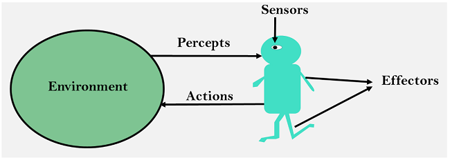
Agent decision making is a crucial aspect of artificial intelligence. It is the process by which an autonomous entity, such as a robot or a computer program, makes decisions based on its available knowledge and perception of the environment. In this post, we will explore the different types of decision making, including simple and complex decisions, as well as sequential decision making, where the agent’s utility depends on a sequence of decisions. We will also discuss the various techniques used in decision making.

Table of Contents

• Making Simple Decisions
  • Utility Theory
  • Multi-Attribute Utility Functions
  • Decision Networks
  • The Value of Information
• Making Complex Decisions
  • Make a sequence of decisions
  • Markov Property

---

Making Simple Decisions

Utility Theory

Remember what we have discussed on utility in the last post Ray - Intelligent Agent Prolegomenon. We can say that a utility function is a function that assigns a value to a state or a run (in this post we more specifically mean a state). Each run will have a probability under which agent will be placed in the given environment. The concept of expected utility is defined as follows: (in this post we will use some simplified notations)

\[EU(A \mid E) = \sum_{i} P(Result_i | E, Do(A)) U(Result_i)\]

The principle of maximizing expected utility is to choose action $A$ with highest $EU(A \mid E)$.

We want our agent to be rational, that is to obey the constraints. And to have behavior describable as maximization of expected utility. To formulate utility theory we need a few more definitions or notations:

Lottery $L$ is a collection of possible outcomes with associated probabilities:

\[L = \{p_1, S_1; p_2, S_2; \ldots; p_n, S_n\} \quad \text{ where } \sum_{i=1}^n p_i = 1\]

Different outcomes (lets say $S_i, S_j$) have following ordering relations:

• $S_i \succ S_j$: $S_i$ is preferred to $S_j$.
• $S_i \succeq S_j$: $S_j$ is not preferred to $S_i$.
• $S_i \sim S_j$: $S_i$ and $S_j$ are indifferent.

The constraints are defined as follows:

• Orderability: $(A \succ B) \vee (B \succ A) \vee (A \sim B)$.
• Transitivity: $(A \succ B) \land (B \succ C) \implies (A \sim C)$.
• Continuity: $(A \succ B \succ C) \implies \exists p \in [0,1] \text{ such that } B \sim pA + (1-p)C$.
• Substitutability: $(A \sim B) \implies {p, A; 1-p, C} \sim {p, B; 1-p, C}$.
• Monotonicity: $(A \succ B) \implies {p, A; 1-p, C} \succ {p, B; 1-p, C}$.
• Decomposability: ${p, A; 1-p, { q, B; 1-q, C } } \sim { p, A; (1-p)q, B; (1-p)(1-q), C }$

Utility Principle can be defined as follows:

\[U(A) > U(B) \implies A \succ B\]

Maximum Expected Utility principle can be defined as follows:

\[U(\{ p_1, S_1; p_2, S_2; \ldots; p_n, S_n \}) = \sum_{i=1}^n p_i U(S_i)\]

Utility functions indicates the goals that the agent’s actions aim to accomplish, which can be determined by analyzing the agent’s preferences. It is a function (mapping) that assigns a value to a state. Considering a complex decision making scenario $A$. The approach to compute utility is to compare to standard lottery $L_p$, and have following definition:

• $U^{\top}$: best possible prize with probability $p$.
• $U^{\bot}$: worst possible penalty with probability $1 - p$.

And we can adjust the $p$ until $A \sim L_p$. On the other hand, we can do some scaling of the utility functions:

• Positive Linear Transform: $U’(x) = k_1 U(x) + k_2 \quad k_1 > 0$
• Normalized utility: $U^{\top} = 1, U^{\bot} = 0$

Multi-Attribute Utility Functions

Multi-Attribute Utility Theory (MAUT) involves evaluating outcomes based on multiple attributes. For instance, when selecting a site for a new airport, factors such as construction disruption, land cost, and noise are taken into account. The approach focuses on identifying patterns in preference behavior. Formally, we have following notation:

Attributes are defined as:

\[X_1, X_2, X_3, \ldots, X_n\]

Combine them to form a Attribute Vector:

\[\boldsymbol{X} = \langle X_1, X_2, X_3, \ldots, X_n \rangle\]

Utility functions can be written as:

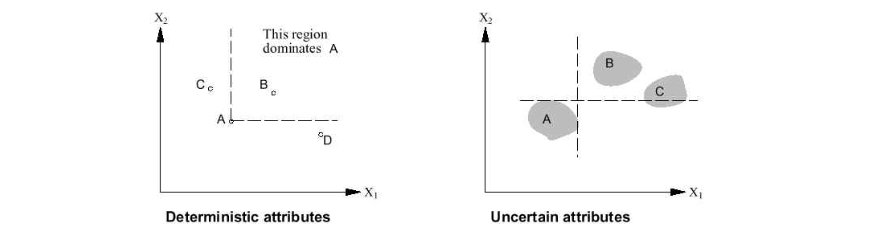
\[U(X_1, X_2, X_3, \ldots, X_n) = f[ f_1(X_1), f_2(X_2), f_3(X_3), \ldots, f_n(X_n) ]\]

The concept of dominance is extended to multi-attribute utility functions. There are two types of dominance:

• Strict Dominance: Take airport $S_1$ and $S_2$ as examples. If site $S_1$ cost less, less noise, safer than $S_2$, we say $S_1$ has strict dominance over $S_2$.
• Stocastic Dominance: In real world, we can not always get the exact value of attributes. The stocastic dominance is the extension of strict dominance to the stocastic case. Say $S_1$ average cost is $3.7$ billion with standard deviation of $0.4$ billion, and $S_2$ average cost is $4.0$ billion with standard deviation of $0.35$ billion. Then $S_1$ has stocastic dominance over $S_2$.

Decision Networks

The Value of Information

---

Making Complex Decisions

Make a sequence of decisions

Components:

• States $s$, starting with the initial state $s_0$
• Actions $a$
• Each state $s$ has a set of actions $A(s)$ that can be taken from it
• Transition model $P(s’ | s, a)$ The Markov assumption states that the probability of transitioning from $s$ to $s’$ when taking action a only depends on the current state s and the action a, and not on any previous actions or states
• Reward function $R(s)$
• Policy π(s): the action that an agent should take in each state
• The “solution” to an MDP

Markov Property

---