Multiagent Decision Making among Self-Interested Agents: Game Theory Foundations

As we delve into the realm of multiagent decision making, game theory emerges as a powerful tool for understanding strategic interactions between self-interested agents. Born from the intersection of economics, mathematics, and computer science, game theory provides a robust framework for analyzing complex decision-making processes. In this post, we’ll embark on an exploration of the game theory foundations that underlie the intricate dance of cooperation and competition among self-interested agents. This journey will cover the essential concepts and theories that form the backbone of Lecture 8 in the SC4003 course at NTU. Buckle up, and let’s dive into the fascinating world of game theory!
Table of Contents
Notations and Definitions
Before we start, let’s have a short definition of game theory notations, which will make the rest of this post easier to understand.
Utilities and Preferences
Say we have two agents:
\[Ag = \{i, j\}\]They are assumed to be self-interested, which means they have preferences over how the environment is. The set of “outcomes” that agents have preferences over is denoted as:
\[\Omega = \{\omega_1, \omega_2, \ldots, \omega_n\}\]We capture preferences by utility functions:
\[U_i: \Omega \to \mathbb{R}, \quad U_j: \Omega \to \mathbb{R}\]Utility functions lead to preference orderings over outcomes:
\[\begin{align*} \omega \succ_i \omega' &\iff U_i(\omega) > U_i(\omega') \\ \omega \succeq_i \omega' &\iff U_i(\omega) \geq U_i(\omega') \\ \end{align*}\]Note that utility is not money, it is a measure of desirability. But it is a useful analogy.
Multiagent Encounters
We need a model of the environment in which these agents will act. Agents simultaneously choose an action in set $Ac$ to perform, and as a result of the actions they select, an outcome $\omega$ in $\Omega$ will result. The actual outcome depends on the combination of actions. Assume each agent has just two possible actions that it can perform, cooperate $C$ and defect $D$. Environment behavior given by state transformer function:
\[\tau: Ac \times Ac \to \Omega\]For convenience, we can also express utility functions as follows. In fact, this notation will be used throughout this post instead of the one above.
\[U_{agent}: Ac \times Ac \to \mathbb{R}\]Classically, we will encounter following situation:
- $\tau(C, C) = \omega_1$, $\tau(C, D) = \omega_2$, $\tau(D, C) = \omega_3$, $\tau(D, D) = \omega_4$: the environment is sensitive to actions of both agents.
- $\tau(C, C) = \omega_1$, $\tau(C, D) = \omega_1$, $\tau(D, C) = \omega_1$, $\tau(D, D) = \omega_1$: neither agent has any influence in this environment.
- $\tau(C, C) = \omega_1$, $\tau(C, D) = \omega_1$, $\tau(D, C) = \omega_2$, $\tau(D, D) = \omega_2$: the environment is sensitive to actions of only one agent.
Rational Action
Suppose we have the case where both agents can influence the outcome, and they have utility functions as follows:
\[U_i(C, C) = 4, \quad U_i(C, D) = 4, \quad U_i(D, C) = 1, \quad U_i(D, D) = 1\] \[U_j(C, C) = 4, \quad U_j(C, D) = 1, \quad U_j(D, C) = 4, \quad U_j(D, D) = 1\]The preferences of agent i are:
\[\langle C, C \rangle \succeq_i \langle C, D \rangle \succ_i \langle D, C \rangle \succeq_i \langle D, D \rangle\]Cooperate is a better choice for $i$, and $i$ will choose cooperate.
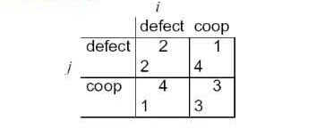
We can characterize the previous scenario in a payoff matrix:

or in a more simplified form:
\[\left( \begin{matrix} (U_i(D, D), U_j(D, D)) & (U_i(C, D), U_j(C, D)) \\ (U_i(D, C), U_j(D, C)) & (U_i(C, C), U_j(C, C)) \end{matrix} \right) = \left( \begin{matrix} (1, 1) & (4, 1) \\ (1, 4) & (4, 4) \end{matrix} \right)\]where agent $i$ is the column player, and agent $j$ is the row player.
Zero-Sum Game and Nonzero-Sum Game
A game is zero-sum if the sum of utilities across all agents for every possible outcome is zero:
\[\forall (ac_i, ac_j) \in Ac \times Ac \rightarrow U_i(ac_i, ac_j) + U_j(ac_i, ac_j) = 0\]or more broadly defined as:
\[\forall \omega \in \Omega \rightarrow \sum_i U_i(\omega) = 0\]An example payoff matrix for a zero-sum game:
\[\left( \begin{matrix} (1, -1) & (-3, 3) \\ (0, 0) & (-4, 4) \end{matrix} \right)\]In this strict competition scenario, pie is fixed. One player win necessarily leads to the other player losing, and vice versa.
A game is non-zero-sum if there exists at least one outcome where utilities do not sum to zero:
\[\exists (ac_i, ac_j) \in Ac \times Ac \rightarrow U_i(ac_i, ac_j) + U_j(ac_i, ac_j) \neq 0\]or more broadly defined as:
\[\exists \omega \in \Omega \rightarrow \sum_i U_i(\omega) \neq 0\]This scenario may allow cooperative outcomes (variable-pie). It is a more general case in the real world. The interesting thing is that zero-sum encounters in real life are very rare, but people tend to act in many scenarios as if they were zero-sum.
Solution Concepts
A rational agent behave in a rational manner in the given scenario according to some strategy derived from previous research. In this section, we will focus on some of them.
Dominant Strategies
Given any particular strategy (either $C$ or $D$) of agent $i$, there will be a number of possible outcomes. We say $s_1$ dominates $s_2$ for $i$ if every outcome possible by $i$ playing $s_1$ is preferred over every outcome possible by $i$ playing $s_2$. A rational agent will never play a dominated strategy.
\[\left( \begin{matrix} (1, 1) & (4, 1) \\ (1, 4) & (4, 4) \end{matrix} \right)\]In previous example, $C$ dominates $D$ for both players. So in deciding what to do, we can delete dominated strategies. Unfortunately, there isn’t always a unique undominated strategy. However, dominant strategy equilibrium can be obtained by each player chooses her dominant strategy.
Nash Equilibrium Strategies
In general, we will say that two strategies $s_1$ (for $i$) and $s_2$ (for $j$) are in Nash equilibrium if:
- under the assumption that agent $i$ plays $s_1$, agent $j$ can do no better than play $s_2$
- under the assumption that agent $j$ plays $s_2$, agent $i$ can do no better than play $s_1$
More mathematically, we say that $s_1$ for agent $i$ and $s_2$ for agent $j$ are in Nash equilibrium if:
\[\neg \exists s_1', s_2' \in Ac \times Ac \text{ s.t. } U_i(s_1', s_2) > U_i(s_1, s_2) \text{ or } U_j(s_1, s_2') > U_j(s_1, s_2)\]Unfortunately, the fact is that:
- Not every interaction scenario has a pure strategy Nash equilibrium.
- Some interaction scenarios have more than one pure strategy Nash equilibrium.
Note that pure strategy here means that each player only choose one action to play. In opposite concept, if each player can choose an action according to a probability distribution, then we call it mixed strategy. Let’s see an example:
Players $i$ and $j$ simultaneously choose the face of a coin, either “heads” or “tails”. If they show the same face, then $i$ wins, while if they show different faces, then $j$ wins. By the way, this is the zero-sum game. And the payoff matrix can be set as:
\[\left( \begin{matrix} (-1, 1) & (1, -1) \\ (1, -1) & (-1, 1) \end{matrix} \right)\]Can tell no pair of strategies forms a pure strategy Nash equilibrium: whatever pair of strategies is chosen, somebody will wish they had done something else. In other words, there is always motivated to change their strategy. To solve this problem, we can play the action under distribution.
Let’s first extend pure strategy Nash equilibrium to mixed strategy Nash equilibrium. The utility of mixed strategy can be expressed as:
\[U_i(\sigma_i, \sigma_j) = \sum_{a_i \in Ac_i} \sum_{a_j \in Ac_j} \sigma_i(a_i) \sigma_j(a_j) \cdot U_i(a_i, a_j).\]where $\Sigma_i$ is player $i$’s mix strategy distribution space, $\sigma_i$ is player $i$’s one mix strategy. Mix strategy pairs $(\sigma_i, \sigma_j)$ are in Nash equilibrium if:
\[\neg \exists \sigma_i', \sigma_j' \in \Sigma_i \times \Sigma_j \text{ s.t. } U_i(\sigma_i', \sigma_j) > U_i(\sigma_i, \sigma_j) \text{ or } U_j(\sigma_i, \sigma_j') > U_j(\sigma_i, \sigma_j)\]Mixed strategies to play “heads” with probability $0.5$ and play “tails” with probability $0.5$ for both players are in Nash equilibrium. This is an example of a mixed strategy Nash equilibrium.
It can be proved that every finite game has a Nash equilibrium in mixed strategies based on fixed point theorem (Brouwer/Kakutani).
Pareto Optimality Strategies
An outcome is said to be Pareto optimal (or Pareto efficient) if there is no other outcome that makes one agent better off without making another agent worse off.
Formally, $\omega$ is said to be Pareto optimal (or Pareto efficient) if there is no other outcome $\omega’$ such that:
\[\begin{align*} & U_i(\omega) \leq U_i(\omega') \\ \text{AND } & U_j(\omega) \leq U_j(\omega') \\ \text{AND } & [U_i(\omega) < U_i(\omega') \text{ OR } U_j(\omega) < U_j(\omega')] \end{align*}\]If an outcome is Pareto optimal, then at least one agent will be reluctant to move away from it (because this agent will be worse off). If an outcome $\omega$ is not Pareto optimal, then there is another outcome $\omega’$ that makes everyone as happy, if not happier, than $\omega$.
In the economic sense:
- Nash equilibrium is the inevitable result of individual rationality, but it may fall into the trap of “collective irrationality”, which require external intervention (such as taxation and agreements).
- Pareto optimality is the ideal state of collective rationality, but it may require forced cooperation or institutional design to achieve it. Through rule design (such as auction rules), Nash equilibrium can be brought close to Pareto optimality.
- The inequality between the two is the core logic of game theory to explain social contradictions (such as the tragedy of the commons and price wars).
Max Social Welfare Strategies
The social welfare (think of it as the “total amount of wealth in the system”) of an outcome $\omega$ is the sum of the utilities that each agent gets from $\omega$:
\[\sum_{i \in Ag} U_i(\omega)\]As a solution concept, may be appropriate when the whole system (all agents) has a single owner (then overall benefit of the system is important, not individuals).
The Prisoner’s Dilemma
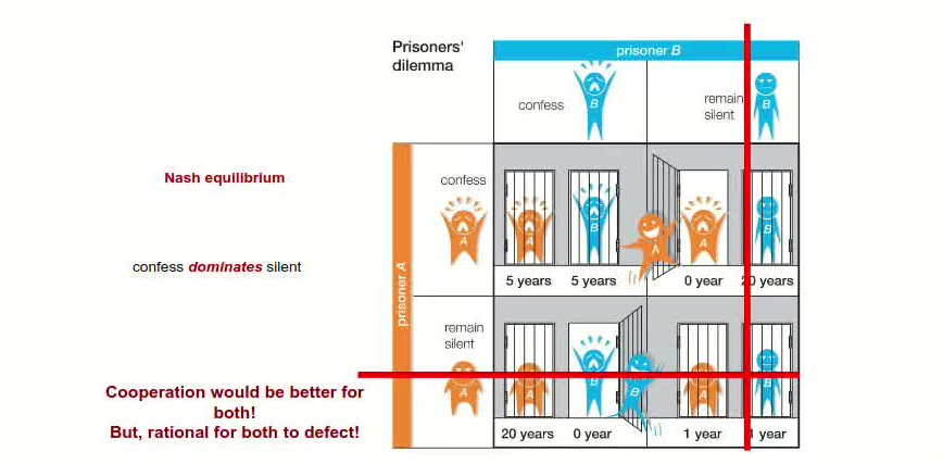
We can assume the following payoff matrix to describe the Prisoner’s Dilemma:
- Top left: If both defect, then both get punishment for mutual defection.
- Top right: If $i$ cooperates and $j$ defects, $i$ gets sucker’s payoff of $1$, while $j$ gets $4$.
- Bottom left: If $j$ cooperates and $i$ defects, $j$ gets sucker’s payoff of $1$, while $i$ gets $4$.
- Bottom right: Reward for mutual cooperation.
The individual rational action is defect which guarantees a payoff of no worse than $2$, whereas cooperating guarantees a payoff of at most $1$. So defection is the best response to all possible strategies: both agents defect, and get payoff $= 2$.
But intuition says this is not the best outcome. Surely they should both cooperate and each get payoff of $3$!
- $D$ is a dominant strategy
- $\langle D,D \rangle$ is the only Nash equilibrium.
- All outcomes except $\langle D,D \rangle$ are Pareto optimal.
- $\langle C,C \rangle$ maximises social welfare.
This apparent paradox is the fundamental problem of multi-agent interactions. It appears to imply that cooperation will not occur in societies of self-interested agents. An example in the real world is the nuclear arms reduction. The core difficulty here is how to recover cooperation.
The strategy we really want to play in the prisoner’s dilemma is that I’ll cooperate if he will. Program equilibria provide one way of enabling this. Each agent submits a program strategy to a mediator which jointly executes the strategies. Crucially, strategies can be conditioned on the strategies of the others.
In The Iterated Prisoner’s Dilemma, If we know we will be meeting our opponent again, then the incentive to defect appears to evaporate. Cooperation is the rational choice in the infinitely repeated prisoner’s dilemma. However, playing the prisoner’s dilemma with a fixed, finite, pre-determined, commonly known number of rounds, defection is the best strategy. This is the backwards induction problem.
Suppose we play iterated prisoner’s dilemma against a range of opponents, what strategy should we choose, so as to maximize our overall payoff? Axelrod (1984) investigated this problem with a computer tournament for programs playing the prisoner’s dilemma. His research suggests the following rules for succeeding:
- Don’t be envious: Don’t play as if it were zero sum!
- Be nice: Start by cooperating, and reciprocate cooperation.
- Retaliate appropriately: Always punish defection immediately, but use “measured” force.
- Don’t hold grudges: Always reciprocate cooperation immediately!
By the way this interesting problem is set to be the assignment, which quiet surprises me.
Related Posts / Websites 👇
📑 Ray - NTU SC4003 Lecture 3 Note: Intelligent Agent Prolegomenon
📑 Ray - NTU SC4003 Lecture 4 Note: Agent Decision Making
📑 Ray - NTU SC4003 Lecture 5 Note: Agent Architecture
📑 Ray - NTU SC4003 Lecture 7 Note: Working Together Benevolent/Cooperative Agents
📑 Ray - NTU SC4003 Lecture 9 Note: Allocating Scarce Resources: Auction
Comments